
Analyzing Data with NumPy
We are studying inflammation in patients who have been given a new treatment for arthritis, and need to analyze the first dozen data sets. The data sets are stored in comma-separated values (CSV) format. Each row holds data for a single patient. The columns represent arthritis inflammations per day on successive days. The first few rows of our first file look like this:
0,0,1,3,1,2,4,7,8,3,3,3,10,5,7,4,7,7,12,18,6,13,11,11,7,7,4,6,8,8,4,4,5,7,3,4,2,3,0,0
0,1,2,1,2,1,3,2,2,6,10,11,5,9,4,4,7,16,8,6,18,4,12,5,12,7,11,5,11,3,3,5,4,4,5,5,1,1,0,1
0,1,1,3,3,2,6,2,5,9,5,7,4,5,4,15,5,11,9,10,19,14,12,17,7,12,11,7,4,2,10,5,4,2,2,3,2,2,1,1
0,0,2,0,4,2,2,1,6,7,10,7,9,13,8,8,15,10,10,7,17,4,4,7,6,15,6,4,9,11,3,5,6,3,3,4,2,3,2,1
0,1,1,3,3,1,3,5,2,4,4,7,6,5,3,10,8,10,6,17,9,14,9,7,13,9,12,6,7,7,9,6,3,2,2,4,2,0,1,1
The master copy of the data for this study is in a git repository. You can browse that repository
here: https://github.com/SWC-OSG-Workshop/ExampleData. Let's take a look. Inside the Python folder are several CSV files. We'll use them in the upcoming examples.
N.B. You can also get a copy of this data in your OSG Connect account by cloning it from github:
$ git clone https://github.com/SWC-OSG-Workshop/ExampleData.git
We want to:
- load the CSV data into memory,
- calculate the average inflammation per day across all patients, and
- plot the result.
To do all that, we'll learn a little bit about programming in Python.
IPython Notebook is a useful tool for interactive data exploration and visualization. An IPython server runs the code, and you interact with it through a web browser. OSG Connect hosts an IPython server for training here: https://ipython.osgconnect.net/swc-duke. Let's go there now. (You will need to log in.)
Once your IPython Notebook application opens, you'll see a list of folders:
dataExampleDataIPython-ExamplesSWC-Pythonusers
ExampleData is a copy of the ExampleData repository mentioned previously. Click on ExampleData, then on Python to "move into" this folder. You won't see the .csv files because they're not Notebook files, but they are present.
Now open a new notebook by clicking on New Notebook in the upper right corner of your IPython Notebook screen.
IPython Notebook follows a command/response pattern that may be familiar to you. In each box marked "In", you will enter Python code. You can enter multiple lines of code in Notebook. When you are done, press SHIFT+ENTER to execute the code you entered. If any output is produced, or if the code you entered returns a value, it will be shown in a box marked "Out".
We'll try this pattern now with a few trivial commands. After each command, press SHIFT+ENTER.
print "hello"
3+5
max(9, 4, 21, 12)
sum([9, 4, 21, 12])
x1, y1 = 1, 1
x2, y2 = 9, 4
slope = (y2 - y1) / (x2 - x1)
slope
Objectives
- Explain what a library is, and what libraries are used for.
- Load a Python library and use the things it contains.
- Read tabular data from a file into a program.
- Assign values to variables.
- Select individual values and subsections from data.
- Perform operations on arrays of data.
- Display simple graphs.
Libraries
The essence of practical programming — as with mathematics — is learning to use fundamental tools and techniques to accomplish more complex tasks, without feeling overwhelmed by the magnitude of the greater task.
Many of powerful tools are built into the core of languages like Python, but as with a volume of mathematical proofs, even more power resides in the libraries that developers build. Different tasks that these libraries implement can be combined sequentially or conditionally to produce programs that do a lot of work, but with relatively simple rules.
In Python, a library is loaded using the import statement. Let's do a simple demonstration by looking for the files in the current folder. (Recall from the section on shell programming that . represents the current directory.) Type the following:
import os
os.listdir('.')
os is a library that implements some useful procedures for interacting with the operating system. listdir is a function, residing in the os library (or "module") which finds all the files in a directory. It returns these as a list that you can assign to a variable, or just display on the screen.
Loading Data
In order to work with our inflammation data, we will import a library called NumPy that knows how to operate on matrices:
import numpy
Importing a library is like getting a piece of lab equipment out of a storage locker and setting it up on the bench. NumPy in particular knows how to read and interpret CSV files, so we can ask it to load our data directly from a file:
numpy.loadtxt(fname='inflammation-01.csv', delimiter=',')
array([[ 0.,  0.,  1., ...,  3.,  0.,  0.],
       [ 0.,  1.,  2., ...,  1.,  0.,  1.],
       [ 0.,  1.,  1., ...,  2.,  1.,  1.],
       ...,
       [ 0.,  1.,  1., ...,  1.,  1.,  1.],
       [ 0.,  0.,  0., ...,  0.,  2.,  0.],
       [ 0.,  0.,  1., ...,  1.,  1.,  0.]])
The expression numpy.loadtxt(...) is a function call that asks Python to run the function loadtxt that belongs to the numpy library. This dotted notation is used everywhere in Python to refer to the parts of things as whole.part.
numpy.loadtxt has two parameters: the name of the file we want to read, and the delimiter that separates values on a line. These both need to be character strings (or strings for short), so we put them in quotes.
When we are finished typing and press Shift+Enter, the notebook runs our command. Since we haven't told it to do anything else with the function's output, the notebook displays it. In this case, that output is the data we just loaded. By default, only a few rows and columns are shown (with ... displayed to mark missing data). To save space, Python displays numbers as 1. instead of 1.0 when there's nothing interesting after the decimal point.
If you want to suppress the output, insert ";" at the end of the statement.
numpy.loadtxt(fname='inflammation-01.csv', delimiter=',');
IPython Notebook continuously saves your work, but you can ask it to save at any time by typing Command-S (Mac) or Control-S (Windows).
Our call to numpy.loadtxt read our file, but didn't save the data in memory. To do that, we need to assign the array to a variable. A variable is just a name for a value, such as x, current_temperature, or subject_id. We can create a new variable simply by assigning a value to it using =:
weight_kg = 55
Once a variable has a value, we can print it:
print weight_kg
55
and do arithmetic with it:
print 'weight in pounds:', 2.2 * weight_kg
weight in pounds: 121.0
We can also change a variable's value by assigning it a new one:
weight_kg = 57.5
print 'weight in kilograms is now:', weight_kg
weight in kilograms is now: 57.5
As the example above shows, we can print several things at once by separating them with commas.
In Python, as in most other common programming languages, assignment refers to the linking of a name (also called a variable, symbol, or label) to a value. It's a simple one-way relation. Assigning a value to one variable does not change the values of other variables.
For example, let's now store the subject's weight in pounds in a variable:
weight_lb = 2.2 * weight_kg
print 'weight in kilograms:', weight_kg, 'and in pounds:', weight_lb
weight in kilograms: 57.5 and in pounds: 126.5
Now let's change weight_kg.
weight_kg = 100.0
print 'weight in kilograms is now:', weight_kg, 'and weight in pounds is still:', weight_lb
weight in kilograms is now: 100.0 and weight in pounds is still: 126.5
Even though we initially defined weight_lb in terms of weight_kg, that relation does not persist, and weight_lb doesn't change when we redefine weight_kg. The conversion of weight_kg to weight_lb happens at the moment that it's assigned, and never again after. The assignment itself is binding. This may feel unnatural, especially if you're used to working with spreadsheets. In a spreadsheet the only way to define one cell in terms of another is through a function. Python has functions too, but they don't look quite the same as assignments. We'll go over these later.
Now that we know how to assign things to variables, let's re-run numpy.loadtxt and save its result:
data = numpy.loadtxt(fname='inflammation-01.csv', delimiter=',')
This statement doesn't produce any output because assignment doesn't return anything — the value previously returned and displayed is now bound up in the variable data.. If we want to check that our data has been loaded, we can print the variable's value:
print data
[[ 0.  0.  1. ...,  3.  0.  0.]
 [ 0.  1.  2. ...,  1.  0.  1.]
 [ 0.  1.  1. ...,  2.  1.  1.]
 ...,
 [ 0.  1.  1. ...,  1.  1.  1.]
 [ 0.  0.  0. ...,  0.  2.  0.]
 [ 0.  0.  1. ...,  1.  1.  0.]]
Manipulating Data
Now that our data is in memory, we can start doing things with it. First, let's ask what type of thing data refers to:
print type(data)
<type 'numpy.ndarray'>
The output tells us that data currently refers to an N-dimensional array created by the NumPy library. We can see what its shape is like this:
print data.shape
(60, 40)
This tells us that data has 60 rows and 40 columns. data.shape is a member of data, i.e., a value that is stored as part of a larger value. We use the same dotted notation for the members of values that we use for the functions in libraries because they have the same part-and-whole relationship.
If we want to get a single value from the matrix, we must provide an index in square brackets, just as we do in math:
print 'first value in data:', data[0, 0]
first value in data: 0.0
print 'middle value in data:', data[30, 20]
middle value in data: 13.0
The expression data[30, 20] may not surprise you, but data[0, 0] might. Programming languages like Fortran and MATLAB start counting at 1, because that's what humans are most accustomed to. Languages in the C family (including C++, Java, Perl, and Python) count from 0 because it's simpler for computers to do, which in turn makes it easier for programmers to sequence multiple steps that deal with the same arrays. (There's a lot less adding or subtracting 1 overall.) As a result, if we have an M×N array in Python, its indices go from 0 to M-1 on the first axis and 0 to N-1 on the second. It takes a bit of getting used to, but one way to remember the rule is that the index is how many steps we have to take from the start to get the item we want.
In the Corner
What may also surprise you is that when Python displays an array, it shows the element with index
[0, 0]in the upper left corner rather than the lower left. This is consistent with the way mathematicians draw matrices, but different from the Cartesian coordinates. The indices are (row, column) instead of (column, row) for the same reason.
Ranges
Python has a standard range notation used to denote slices or subsets of a set. Any array in Python can be sliced using range notation. As an example, suppose we have a set of children's ages:
ages = [2, 3, 6, 9, 11, 13, 17]
Range notation causes ages[1:4] to refer to elements 1, 2, and 3 of the list — the slice starting at index 1 and extending to (but not including) index 4 — or [3, 6, 9]. The 1 is the index of the start of the range, and the 4 — counterintuitively —is the index of the item after the last item in the subset. So elements N through M of a set named "sequence" would be indicated as sequence[N:M+1]. It is also possible to leave out the N or M values.
Since character strings are a kind of array, this is most easily demonstrated using strings:
soup = "french onion"
print soup[4:9]
print soup[:6]
print soup[7:]
NumPy's N-Dimensional Ranges
An index like [30, 20] selects a single element of an array, but we can select whole sections as well, using an extended form of range notation. For example, we can select the first ten days (columns) of values for the first four (rows) patients like this:
print data[0:4, 0:10]
[[ 0.  0.  1.  3.  1.  2.  4.  7.  8.  3.]
 [ 0.  1.  2.  1.  2.  1.  3.  2.  2.  6.]
 [ 0.  1.  1.  3.  3.  2.  6.  2.  5.  9.]
 [ 0.  0.  2.  0.  4.  2.  2.  1.  6.  7.]]
The slice 0:4 means, "Start at index 0 and go up to, but not including, index 4." Again, the up-to-but-not-including takes a bit of getting used to, but the rule is that the difference between the upper and lower bounds is the number of values in the slice.
We don't have to start slices at 0:
print data[5:10, 0:10]
[[ 0.  0.  1.  2.  2.  4.  2.  1.  6.  4.]
 [ 0.  0.  2.  2.  4.  2.  2.  5.  5.  8.]
 [ 0.  0.  1.  2.  3.  1.  2.  3.  5.  3.]
 [ 0.  0.  0.  3.  1.  5.  6.  5.  5.  8.]
 [ 0.  1.  1.  2.  1.  3.  5.  3.  5.  8.]]
and we don't have to take all the values in the slice---if we provide a stride, Python takes values spaced that far apart:
print data[0:10:3, 0:10:2]
[[ 0.  1.  1.  4.  8.]
 [ 0.  2.  4.  2.  6.]
 [ 0.  2.  4.  2.  5.]
 [ 0.  1.  1.  5.  5.]]
Here, we have taken rows 0, 3, 6, and 9, and columns 0, 2, 4, 6, and 8. (Again, we always include the lower bound, but stop when we reach or cross the upper bound.)
We also don't have to include the upper and lower bound on the slice. If we don't include the lower bound, Python uses 0 by default; if we don't include the upper, the slice runs to the end of the axis, and if we don't include either (i.e., if we just use ':' on its own), the slice includes everything:
small = data[:3, 36:]
print 'small is:'
print small
small is:
[[ 2.  3.  0.  0.]
 [ 1.  1.  0.  1.]
 [ 2.  2.  1.  1.]]
Arrays also know how to perform common mathematical operations on their values. If we want to find the average inflammation for all patients on all days, for example, we can just ask the array for its mean value.
print data.mean()
6.14875
mean is a method of the array, i.e., a function that belongs to it in the same way that the member shape does. If variables are nouns, methods are verbs: they are what the thing in question knows how to do. This is why data.shape doesn't need to be called (it's just a thing) but data.mean() does (it's an action). It is also why we need empty parentheses for data.mean(): even when we're not passing in any parameters, parentheses are how we tell Python to go and do something for us.
NumPy arrays have lots of useful methods:
print 'maximum inflammation:', data.max()
print 'minimum inflammation:', data.min()
print 'standard deviation:', data.std()
maximum inflammation: 20.0
minimum inflammation: 0.0
standard deviation: 4.61383319712
When analyzing data, though, we often want to look at partial statistics, such as the maximum value per patient or the average value per day. One way to do this is to select the data we want to create a new temporary array, then ask it to do the calculation:
patient_0 = data[0, :] # 0 on the first axis, everything on the second
print 'maximum inflammation for patient 0:', patient_0.max()
maximum inflammation for patient 0: 18.0
We don't actually need to store the row in a variable of its own. Instead, we can combine the selection and the method call:
print 'maximum inflammation for patient 2:', data[2, :].max()
maximum inflammation for patient 2: 19.0
Note that this is effectively the same mechanism as shell pipelines. You can call methods on top of methods so long as those methods return valid Python objects, without needing to assign these intermediary objects to variables.
What if we need the maximum inflammation for all patients, or the average for each day? As the diagram below shows, we want to perform the operation across an axis:

To support this, most array methods allow us to specify the axis we want to work on. If we ask for the average across axis 0, we get:
print data.mean(axis=0)
[  0.           0.45         1.11666667   1.75         2.43333333   3.15
   3.8          3.88333333   5.23333333   5.51666667   5.95         5.9
   8.35         7.73333333   8.36666667   9.5          9.58333333
  10.63333333  11.56666667  12.35        13.25        11.96666667
  11.03333333  10.16666667  10.           8.66666667   9.15         7.25
   7.33333333   6.58333333   6.06666667   5.95         5.11666667   3.6
   3.3          3.56666667   2.48333333   1.5          1.13333333
   0.56666667]
As a quick check, we can ask this array what its shape is:
print data.mean(axis=0).shape
(40,)
The expression (40,) tells us we have an N×1 vector, so this is the average inflammation per day for all patients. If we average across axis 1, we get:
print data.mean(axis=1)
[ 5.45   5.425  6.1    5.9    5.55   6.225  5.975  6.65   6.625  6.525
  6.775  5.8    6.225  5.75   5.225  6.3    6.55   5.7    5.85   6.55
  5.775  5.825  6.175  6.1    5.8    6.425  6.05   6.025  6.175  6.55
  6.175  6.35   6.725  6.125  7.075  5.725  5.925  6.15   6.075  5.75
  5.975  5.725  6.3    5.9    6.75   5.925  7.225  6.15   5.95   6.275  5.7
  6.1    6.825  5.975  6.725  5.7    6.25   6.4    7.05   5.9  ]
which is the average inflammation per patient across all days.
Challenges
As we previously saw, we can take slices of a character string. For example:
element = 'oxygen'
print 'first three characters:', element[0:3]
print 'last three characters:', element[3:6]
first three characters: oxy
last three characters: gen
What is the value of
element[:4]? What aboutelement[4:]? Orelement[:]?What is
element[-1]? What iselement[-2]? Given those answers, explain whatelement[1:-1]does.The expression
element[3:3]produces an empty string, i.e., a string that contains no characters. Ifdataholds our array of patient data, what doesdata[3:3, 4:4]produce? What aboutdata[3:3, :]?
Plotting
The mathematician Richard Hamming once said, "The purpose of computing is insight, not numbers," and the best way to develop insight is often to visualize data. Visualization deserves an entire lecture (or course) of its own, but we can explore a few features of Python's matplotlib here. First, let's tell the IPython Notebook that we want our plots displayed inline, rather than in a separate viewing window:
%matplotlib inline
The % at the start of the line signals that this is a command for the notebook, rather than a statement in Python. Next, we will import the pyplot module from matplotlib and use two of its functions to create and display a heat map of our data:
from matplotlib import pyplot
pyplot.imshow(data)
pyplot.show()
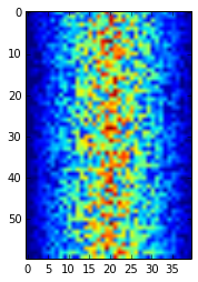
Blue regions in this heat map are low values, while red shows high values. As we can see, inflammation rises and falls over a 40-day period. Let's take a look at the average inflammation over time:
ave_inflammation = data.mean(axis=0)
pyplot.plot(ave_inflammation)
pyplot.show()
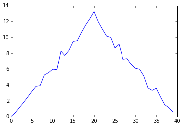
Here, we have put the average per day across all patients in the variable ave_inflammation, then asked pyplot to create and display a line graph of those values. The result is roughly a linear rise and fall, which is suspicious: based on other studies, we expect a sharper rise and slower fall. Let's have a look at two other statistics:
print 'maximum inflammation per day'
pyplot.plot(data.max(axis=0))
pyplot.show()

print 'minimum inflammation per day'
pyplot.plot(data.min(axis=0))
pyplot.show()
maximum inflammation per dayminimum inflammation per day
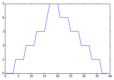
The maximum value rises and falls perfectly smoothly, while the minimum seems to be a step function. Neither result seems particularly likely, so either there's a mistake in our calculations or something is wrong with our data.
Challenges
Why do all of our plots stop just short of the upper end of our graph?
Create a plot showing the standard deviation of the inflammation data for each day across all patients. (Hint: the function standard deviation function is std() )
Wrapping Up
It's very common to create an alias for a library when importing it in order to reduce the amount of typing we have to do. Here are our three plots side by side using aliases for numpy and pyplot:
import numpy as np
from matplotlib import pyplot as plt

data = np.loadtxt(fname='inflammation-01.csv', delimiter=',')

plt.figure(figsize=(10.0, 3.0))

plt.subplot(1, 3, 1)
plt.ylabel('average')
plt.plot(data.mean(0))

plt.subplot(1, 3, 2)
plt.ylabel('max')
plt.plot(data.max(0))

plt.subplot(1, 3, 3)
plt.ylabel('min')
plt.plot(data.min(0))

plt.tight_layout()
plt.show()
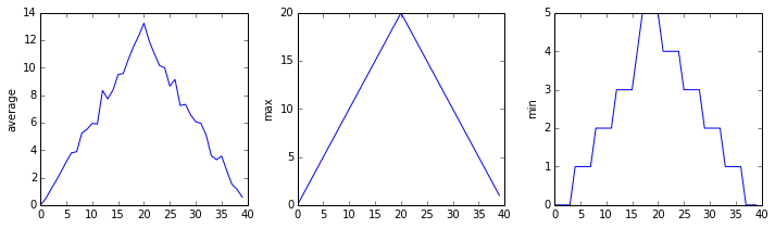
The first two lines re-load our libraries as np and plt, which are the aliases most Python programmers use. The call to loadtxt reads our data, and the rest of the program tells the plotting library how large we want the figure to be, that we're creating three sub-plots, what to draw for each one, and that we want a tight layout. (Perversely, if we leave out that call to plt.tight_layout(), the graphs will actually be squeezed together more closely.)
Challenges
- Modify the program to display the three plots on top of one another instead of side by side. (Hint: subplot(col, row, index starts from 1) )
Key Points
- Import a library into a program using
import libraryname. - Use the
numpylibrary to work with arrays in Python. - Use
variable = valueto assign a value to a variable in order to record it in memory. - Variables are created on demand whenever a value is assigned to them.
- Use
print somethingto display the value ofsomething. - The expression
array.shapegives the shape of an array. - Use
array[x, y]to select a single element from an array. - Array indices start at 0, not 1.
- Use
low:highto specify a slice that includes the indices fromlowtohigh-1. - All the indexing and slicing that works on arrays also works on strings.
- Use
# some kind of explanationto add comments to programs. - Use
array.mean(),array.max(), andarray.min()to calculate simple statistics. - Use
array.mean(axis=0)orarray.mean(axis=1)to calculate statistics across the specified axis. - Use the
pyplotlibrary frommatplotlibfor creating simple visualizations.
Next Steps
Our work so far has convinced us that something's wrong with our first data file. We would like to check the other 11 the same way, but typing in the same commands repeatedly is tedious and error-prone. Since computers don't get bored (that we know of), we should create a way to do a complete analysis with a single command, and then figure out how to repeat that step once for each file. These operations are the subjects of the next two lessons.