Introduction to Open Science Grid
The Open Science Grid
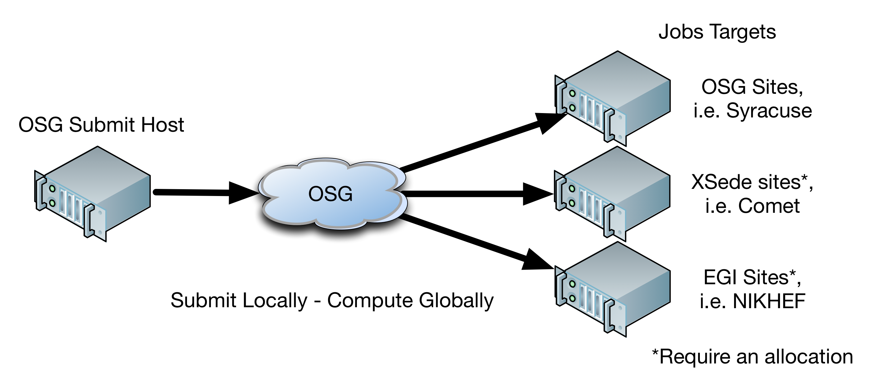
The Open Science Grid (OSG) is a consortium of research communities which facilitates distributed high throughput computing for scientific research. The OSG
- Enables distributed computing on more than 120 institutions (for additional detail and geographic distribution of sites, check the Introduction to OSG slides),
- Supports efficient data processing, and
- Provides large scale scientific computing of 2 million core CPU hours per day.
The OSG provides the unused compute resources at the various OSG contributors opportunistically in an shared pool to outside researchers. This means that resource availability may vary greatly with time.
Computation that is a good match for OSG
High throughput work flows with simple system and data dependencies are a good fit for OSG. Typically, these work flows can be broken down into multiple tasks that can be carried out independently. Ideally, these tasks will download input data, run some computation on it and then return results (which may be used by future tasks).
Jobs submitted into the OSG will be executed on machines at several remote physical clusters. These machines may differ in terms of computing environment from the submit node. Therefore it is important that the jobs are as self-contained as possible. The necessary binaries (and/or scripts) and data should either carried with the job, or staged on demand.
Please consider the following guidelines:
- Software should preferably be single threaded, using less than 2 GB memory and each invocation should run for 1-12 hours (optimally under 3 hours). There is some support for jobs with longer run time, more memory or multi-threading support. Please contact the user support listed below for more information about these capabilities.
- Only core utilities can be expected on the remote end. There is no standard version of software such as
gcc,python,BLAS, or others. Consider using Distributed Environment Modules to manage software dependencies, or read our Developing High-Throughput Applications Guide. - No shared file system. Jobs must transfer all executables, input data, and output data. Input and output data for each job should be < 10 GB to allow them to be transferred in by the jobs, processed and returned to the submit node. The scheduler, HTCondor, can transfer the files for you. Depending on the size of your input and output files, other transfer methods (
scp,rsync,GridFTP) may be better suited. Please contact the user support listed below for more information
Computation that is NOT a good match for OSG
The following are examples of computations that are NOT good matches for OSG:
- Tightly coupled computations, for example using MPI-based communication, will not work well on OSG due to the distributed nature of the infrastructure.
- Computations requiring a shared file system will not work, as there is no shared file system between the different clusters on the OSG.
- Computations requiring complex software deployments or proprietary software are not a good fit. There is limited support for distributing software to the compute clusters, but for complex software, or licensed software, deployment can be a major task.
How to get help using OSG
Please contact user support staff at user-support@opensciencegrid.org.
Available Resources on OSG
Commonly used software and libraries on the Open Science Grid are available in a central repository (known as OASIS) and accessed via the module command. We will see how to search for, load, and use software modules. This command may be familiar to you if you have used HPC clusters before such as XSede's Comet or NERSC's Cori.
We will also cover the usage of the built-in tutorial command. Using tutorial, we load a variety of job templates that cover basic usage, specific use cases, and best practices.
Software Applications
To take a look at the module command, log in to the submit host via SSH:
$ ssh username@training.osgconnect.net
Once you are logged in, you can check the available modules:
$ module avail

[...]
   ANTS/1.9.4                  dmtcp/2.5.0                lapack/3.5.0                     protobuf/2.5
   ANTS/2.1.0           (D)    ectools                    lapack/3.6.1              (D)    psi4/0.3.74
   MUMmer3.23/3.23             eemt/0.1                   libXpm/3.5.10                    python/2.7        (D)
   OpenBUGS/3.2.3              elastix/2015               libgfortran/4.4.7                python/3.4
   OpenBUGS-3.2.3/3.2.3        espresso/5.1               libtiff/4.0.4                    python/3.5.2
   R/3.1.1              (D)    espresso/5.2        (D)    llvm/3.6                         qhull/2012.1
   R/3.2.0                     ete2/2.3.8                 llvm/3.7                         root/5.34-32-py34
   R/3.2.1                     expat/2.1.0                llvm/3.8.0                (D)    root/5.34-32
   R/3.2.2                     ffmpeg/0.10.15             lmod/5.6.2                       root/6.06-02-py34 (D)
   R/3.3.1                     ffmpeg/2.5.2        (D)    madgraph/2.1.2                   rosetta/2015
   R/3.3.2                     fftw/3.3.4-gromacs         madgraph/2.2.2            (D)    rosetta/2016-02
   RAxML/8.2.9                 fftw/3.3.4          (D)    matlab/2013b                     rosetta/2016-32   (D)
   SeqGen/1.3.3                fiji/2.0                   matlab/2014a                     ruby/2.1


[...]

 Where:
   (D):  Default Module

Use "module spider" to find all possible modules.
Use "module keyword [key1 key2...]" to search for all possible modules matching any of the "keys".
In order to load a module, you need to run module load [modulename]. If you want to load the R package,
$ module load R
This sets up the R package for you. Now you can do some test calculations with R.
# invoke R
$ R
# simple on-screen calculation with cosine function
> cos(45)
[1] 0.525322
If you want to unload a module, type
$ module unload R
Tutorial Command
The built-in tutorial command assists a user in getting started on OSG. To see the list of existing tutorials, type
# will print a list tutorials
$ tutorial
Say for example, you are interested in learning how to run R scripts on OSG, the
tutorial command sets up the R tutorial for you.
$ tutorial R
# prints the following message:
Installing R (master)...
Tutorial files installed in ./tutorial-R.
Running setup in ./tutorial-R...
The tutorial R command creates a directory tutorial-R containing the necessary script and input files.
# The example R script file
mcpi.R
# The job execution file
R-wrapper.sh
# The job submission file (will discuss later in the lesson HTCondor scripts)
R.submit
Lets focus on mcpi.R and the R wrapper scripts. The details of R.submit script will be discussed later when we learn about submitting jobs with HTCondor.
The file mcpi.R is a R script that calculates the value of pi using the Monte Carlo method. The R-wrapper.sh essentially loads the R module and runs the mcpi.R
script.
#!/bin/bash

EXPECTED_ARGS=1

if [ $# -ne $EXPECTED_ARGS ]; then
  echo "Usage: R-wrapper.sh file.R"
  exit 1
else
  source /cvmfs/oasis.opensciencegrid.org/osg/modules/lmod/current/init/bash
  module load R
  Rscript $1
fi
There are other tutorials available, which can serve as templates to develop your own scripts to run your workloads on OSG.